Methodology

The analysis was divided into three separate sections:

(Click on the shortcuts to go to the direct section)

Distribution of Amanita phalloides in Vancouver

In order to construct the map of the distribution of current Amanita phalloides, ArcGIS Online was used.

Adding Amanita phalloides sites

To do so, it was necessary to filter the initial document received by Vivian, and to combine the civic number with the street address, and to add new fields such as province name, in order for the software to map each location on the interactive map.

Adding Flourishing number

It was necessary to add UBC's accession Flourishing reference since each Death Cap site recorded was based on Tree IDs and specimen vouchers. The fruiting numbers were added to the excel table of Bellutus trees with sitings, and 2 other sites from other tree species were as well added in order to be mapped.

Adding qualitative data

In addition, relevant qualitative data was collected from the Open Data Catalogue of the City of Vancouver and added as a layer to the map. The layers downloaded as CVS files included: schools, community centres, and community gardens and food trees.

Adding tree data

Adding the tree data to the interactive map required the use of ArcMap. Indeed, the file size was too big to be uploaded online. Consequently, it was necessary to "Select by Attributes" for each different size class of the Betulus file, and to create new layers from the selected features. This was done for the 5 classes present in the data file (S,M,L,V,N, and Blank entries).

The different layers were exported as shapefiles, zipped, and added online to ArcGIS.

The map, which can be seen in the "Results" tab, is interactive, with pop up windows that include relevant information about each Amanita phalloides recorded site. From the map itself, it is possible to click and unclick on the other school and community centre layers.

Note: the original file contained many entries with the option to select only the sites recorded. The 61 sites from the Bellutus trees were copied and pasted into another document and only relevant information was kept, as well as addresses combined, as well as non-belutus sites added. If new sites were to be recorded, updating the interactive map would be relatively easy. New sites would have to be added to both files, and an updated table would be used to upload in ArcMap Online, and easily update the locations. Moreover, as requested by the supervisor, the possibility of adding Flourishing numbers to each tree IDs is made easy.

The excel file used to input into ArcGIS can be found by clicking on the following icon:

- Making the interactive map -
Click on image to enlarge

Buffer and Schools within 500 meters

In addition to displaying the distribution of the mushroom sites across Vancouver with their associated flourishing numbers.
Dissolved buffers of 500m were calculated around the sites of the death caps, and the school layer was clipped to those areas in order to create a new layer with only the schools within 500 meters of the respective sites.
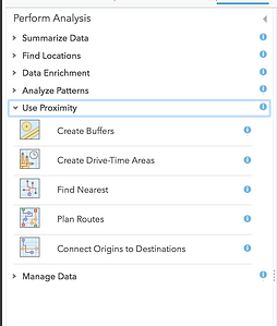
The analysis was possible to be carried out on the online ArcGIS using "Create Buffers" in the "Use Proximity" toolbox
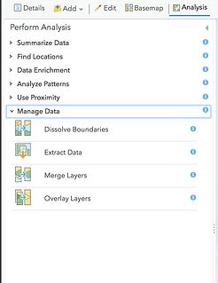
The "Extract Data" in the "Manage Data" toolbox was used to isolate and clip the schools within the 500m buffers.
A screenshot of the analysis can be seen below.

Multi-Criteria Evaluation analysis

For Vancouver - Predicting distribution of the Death Cap

1. Overview

The goal of the MCE for this project was to identify high-risk zones based on proximity to host tree factors and demographic factors. In the context of this analysis, risk is defined as the potential for Amanita phalloides fruition presence and human/dog consumption. Amanita phalloides has shown to have an optimal symbiotic relationship with numerous host trees including Carpinus betulus, Quercus robur, Quercus garryana, Quercus rubra, Castanea sativa, Fagus sylvatica, Corylus avellane, and Tilia species. As this relationship is an example of ectomycorrhizae, the Amanita phalloides fruition occurs at the tip of tree roots, which can be a significant distance from the trunk of the tree. For this reason, the Vancouver tree dataset was first reduced to only the known host tree species listed above and a 50m buffer was applied to each tree location to encompass all of the most likely areas that Amanita phalloides could be found. Once this was achieved, the following list of factors were inputed as vector layers into the ArcMap file:

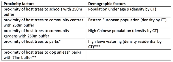
* there is no Vancouver tree data for the parks in Vancouver, so the overlap of the 50m buffer for known host trees with the parks polygons was calculated by clipping the layers. There is some overlap with these layers because some of the parks are bordered by streets that are home to host trees. For overlay percentages greater than 1%, the percentage cover was estimated by the GIS analyst for the following parks: Memorial South Park, Thornton Park, Falaise Park, Morton Park, Delamont Park, Rosemary Brown Park, Jericho Beach Park, Strathcona Linear Park.

** the only retrievable dog park data accessible through the city of Vancouver data catalogue was point data for each dog park location. After inspection of numerous dog parks through Google Maps, it was decided that a buffer of 75m was a fair representation of most of the dog parks in Vancouver. This is a noteworthy assumption but was required in order to conduct the MCE analysis.

*** as no lawn watering data was easily attainable, percentage residential zone land per census tract area was used as a proxy for lawn watering. For example, census tracts with greater residential area coverage were considered to have greater lawn watering and thus could potentially be areas of longer fruition seasons and therefore greater risk.

Once all of the data was collected, each factor was normalized and assigned a weight. The weighted sum tool was used for the proximity factors and demographic factors separately and then also to combine the two weighted sum outputs. This final weighted sum output highlights the risk zones associated with all of the discussed factors and their respective weights.

2. Data Preparation

A - Data Collection

Apart from the data for the factors listed above, the other important data set used was the Vancouver city wide tree database from the datacatalogue. The community centre, community garden and school data points were retrieved through the UBC Geography department computer lab database. As these factors were represented as point data in their original data formats, buffer zones of 250m were applied to these three factors to encompass the entire area where children and/or uninformed community gardeners may pluck and consume. Vancouver park vector polygons and off-leash dog park point locations were imported from the Vancouver data catalogue. The Vancouver park data does not have any tree data attached; for this reason, the overlap of the host tree 50m buffer layers with parks was used to determine the risk associated with each park throughout Vancouver. As the off-leash dog park data is downloadable only as point data, reference to Google Map imagery of the dog parks suggested that a 75m buffer of the Vancouver data catalogue points would be an adequate representation of dog park area for the majority of the dog parks in Vancouver.

For the demographic factor data, the 2016 census data from statcan.gc.ca was used. This included the factor data for population of children under age 9, Chinese population and Eastern European population. The census tract boundary files were downloaded as vector files from statcan.gc.ca, however the census tract factor data could only be downloaded as excel data. So, the excel table data was joined to the census tract boundary data by the common attribute field: census tract ID. To determine the lawn watering data a combination of Vancouver land use data was combined with the census tract boundaries. The Vancouver land use data included residential zoned land which was extracted then compared to the census tract area. The census tract areas with greater residential area coverage were considered to have greater lawn watering and therefore greater risk of presence.

B - Normalization of Factors

In order to normalize/standardize all of the factor data, a field with values of 0 to 10, where 10 means the highest risk, was added to the attribute table of each factor. This field was calculated differently for the proximity factors than for the demographic factors, but the resultant range of values was the same to ensure standardization. For the proximity factors, the area of overlay between each factor and the host tree 50m buffer layer was determined by clipping the data. Then, the area of overlap was divided by the area of each factor location to determine a tree host percentage cover value for each community centre, community garden and school location. To standardize these percentage cover values, these values were divided by the maximum value then multiplied by 10 to ensure a range of values from 0 to 10. For the population demographic factors, the number of people in each study group (age under 9, Chinese or Eastern European) was divided by census tract area to attain percentage of study group population per CT value. Similarly to the proximity factor standardization, these values were then divided by the maximum percentage and multiplied by 10 to ensure a range of values from 0 to 10. The lawn watering data was standardized by dividing the total residential area within a census tract area by the area of that specific census tract then multiplying that value by 10 to ensure a range of values from 0 to 10.

3. Weighting of Factors

The weighting of the factors was the most challenging and arbitrary aspect to the MCE. Are demographic factors more important than proximity factors? Are young children at greater risk than dogs? Does lawn watering affect the risk zones at all? These are the sorts of questions that were thought about when developing the weighting regimes. As there were two clear groups of data type, proximity data, and demographic data, it made sense to execute a weighted sum for each group of factors and then together. In this analysis, the weighted sum was conducted with equal weights and with varying weighting regimes. Some main features of the weighting regimes include:

greater importance for proximity factors (80%) than demographic factors (20%)
greater importance for proximity of host trees to schools (30% or 50%) than all other proximity factors
greater importance for population under age 9 (40% or 50%) than all other demographic factors
weighted sums that include lawn watering as a factor vs. weighted sums without lawn watering considered as a factor

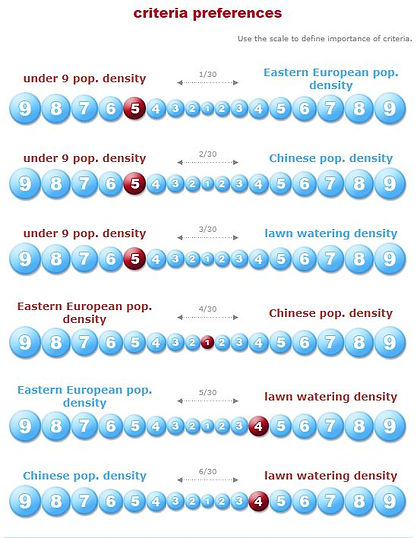
4. Analytical Hierarchy Process

The Analytical Hierarchy Process (AHP) is a way of analyzing complex decisions. In the context of this report, the AHP process was used to determine the weights for each demographic and proximity factor considered. The online software program from 123ahp.com was used to derive the AHP weighting regime that was applied for the final output MCE. The results of the 123ahp derivation are shown below.

Demographic Factors - criteria preferences Demographic Factors - AHP weighting regime

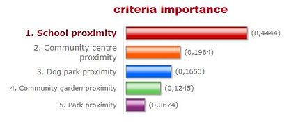
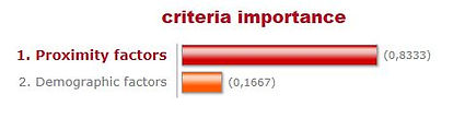
Proximity Factors - criteria preferences Proximity Factors - AHP weighting regime

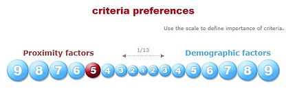
Combination of Factors - criteria preference Combination of Factors - AHP weighting regime

NOTE: Probably the most important criteria preference to note from the above images is the 'Combination of Factors - criteria preference' because this preference assigns much greater importance to the Proximity Factors than the Demographic Factors.

5. Weighted Linear Overlay (Weighted Sum)

Although the process of standardizing all of the factor data was laborious, further transformations of the data layers was required before the 'weighted sum' tool could be used. All of the factors prior to this point were stored as vector layers, but the weighted sum tool requires that all input layers are raster. To convert the proximity factors to raster layers, the 'polygon to raster' tool was used, but a further complication became evident after running this tool – the large areas between the polygons did not have any assigned values. In order to make the raster layers continuous across the Vancouver boundary the 'mosaic to new raster' tool was used. Before using this tool, the Vancouver boundary vector layer was converted to a raster layer that was continuous across the entire city boundary. Now, by including the Vancouver boundary raster layer as well as each factor layer (one by one) as the input layers for the 'mosaic to new raster' tool, the output was a continuous raster. But the output rasters did not carry over the attribute tables of each of the vector layers, so the tables had to be joined by common attribute and then, to ensure that the cells between the polygons were registered as 0 (or, no risk), the normalization values were recalculated. It should be noted that the cell size for all raster layers was set as 1.

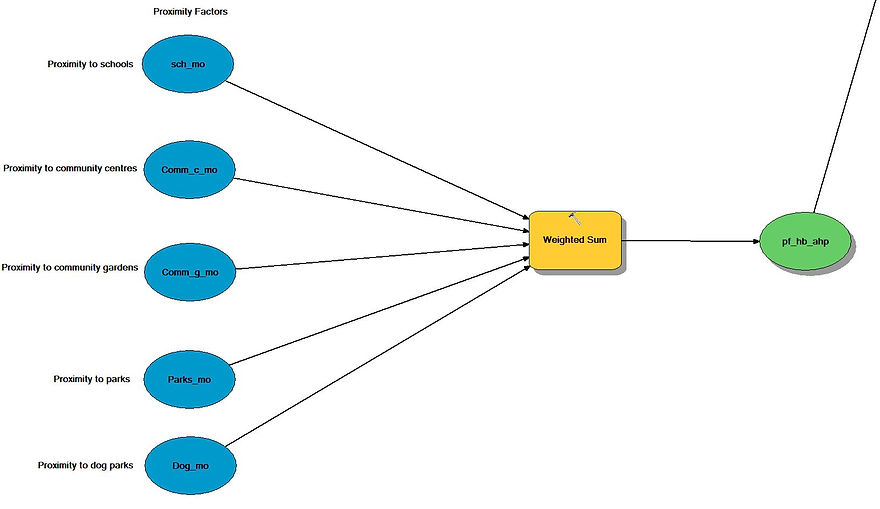
6. Modelbuilder

Modelbuilder was used in ArcMap to execute multiple MCEs with different weighting regimes to increase the output speed, ensure consistency and attain sensitivity analysis outputs. Because of the varying range of MCEs, three models were designed and stored in an ArcMap toolbox. The screenshots below show one of the three models, all models followed this structure. The MCE inputs changed amongst the three models.

Part 1 - Demographic Factors

Part 2 - Proximity Factors

Part 3 - Combination of Demographic Factors and Proximity Factors

Complete model

Maxent Analysis for GVRD (Metro Vancouver)
Prediction of future locations

1. Gather Data

Data was gathered from WorldClim, Cgiar, Vancouver Open Data, the UBC geography labs, and the Centre for Disease Control via Vivian Mao.

2. Sort Data for Maxent

All of the data was then sorted and converted into the appropriate format to be used in Maxent.

Maxent requires that all environmental layers entered into the model have the same cell size, extent, and projection. To begin the process of converting the raster, .tiff, and polygon files into .ASC files I set the processing environment in ArcMap. An initial raster was created using the BC landmass file and the first temperature .tiff from WorldClim. This raster was used to define processing extent, coordinate system, cell size, raster mask, and set as the snap raster to ensure all subsequent rasters were identical. From there every single layer was clipped to the BC landmass and then exported as a .asc file.
Our point data for the occurrence of the Death Cap mushroom just needed to be simplified and converted to a .csv file. Every row except for the tree species name and the longitude and then latitude were deleted. The file was then saved and added into Maxent. The same process was applied for the map showing the top 6 host tree species.
To create the sample species for the Mission and Victoria maps, points were dropped in google maps. The longitude and latitude coordinates were then taken and entered into a .csv file that could be uploaded into Maxent. For the Mission sample, the location of Mission was used as the sample point. For the Victoria samples, the locations as mentioned in the Vancouver Sun report were used.

3. Visualize Data

The .asc files that maxent produced were then uploaded back into ArcMap where the final visualization took place. In ArcMap legends, colour, and information were all added.

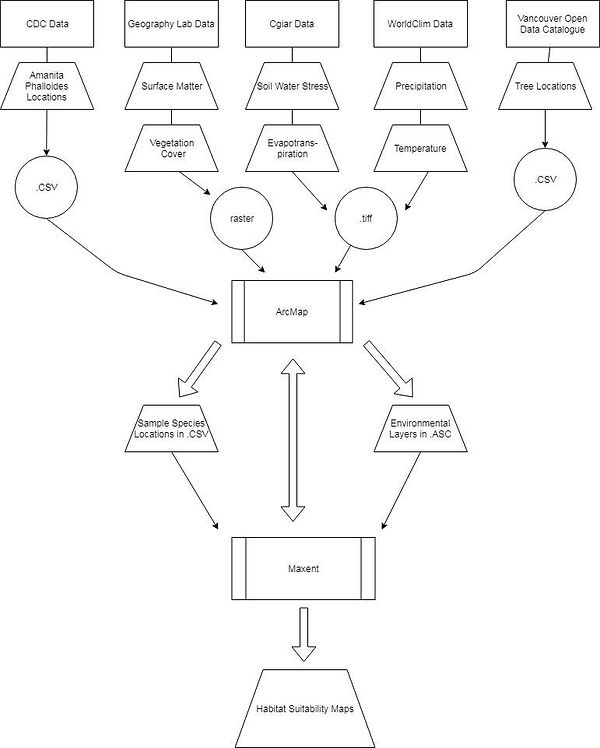
A flowchart of the methodology for the maxent analysis can be seen below:

Distribution Map

MCE

MaxEnt